|
|
|
|
News The Project Technology RoboSpatium Contribute Subject index Download Responses Games Gadgets Contact <<< Current, voltage Rover No.1 >>> OscilloscopeThe videos about oscilloscopesVarying signals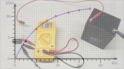
At the previous chapter we learned how to measure constant voltages and currents using digital multimeters. With the help of that measuring instrument you are able to capture no more than a few values per minute. You can examine variable voltages, by doing measurements at given times, but this proceeding makes sense only if the voltage changes slowly over time. How can the number of captured values per minute be increased? Well, the limiting factor is the timespan needed to read the display. This problem can be fixed by displaying the values as a X/Y plot instead of single digital numbers. The Y axis of this two dimensional graph represents the input voltage which is plotted as a function of time at the X axis. Measuring instruments of that type are called Oscilloscopes or short O-scope respectively scope. Oscilloscopes are used to record varying signals, displaying the voltage at the vertical axis. In order to measure other quantities but voltages, the input signal has to be converted into an equivalent potential. For example a current can be transformed into a voltage using a shunt resistor, temperatures can be converted by a thermocouple. Varying signals can occur as a single event or as a periodically changing signal. A single event of a fastly changing signal is a clap with your hands. That sound can be transformed into a varying voltage using a microphone. A slowly changing single event is the temperature profile of one day. Time based plot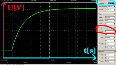
The oscilloscope plot shows the charging procedure of a 22μF capacitor through a 12kΩ resistor at a 12V Battery. The horizontal axis represents the time, while the voltage is allocated to the vertical axis. The resulting plot is a curve with a high slope at the beginning (left) of the procedure and a low slope at the end (right). 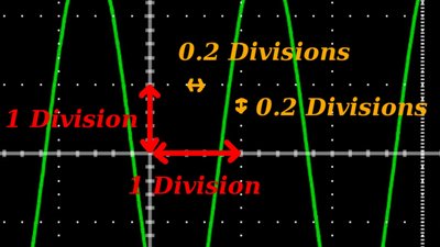
The coordinate system of the graph is represented by a dot-line printed grid. The base unit of the grid is one division, which corresponds the edge of a single rectangle. Each division is sub-divided by 5 dots, hence one dot equals 0.2 divisions. The equivalence of one division can be read respectively adjusted using the dropdown lists to the right of the computer screen. The adjustment of the horizontal axis is also named timebase or Sweep. 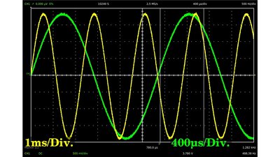
The input signal is displayed with different horizontal adjustments (in a single plot using GIMP image manipulation): The green curve is recorded with a timebase of 400μs/Div, the yellow curve using 1ms/Div. The reading for a period is 5.8 divisions at the green and 2.9 divisions at the yellow curve. The resulting period is identically for both curves: 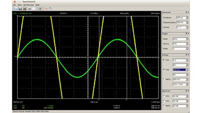
Even if the peaks of the yellow curve are out of range, you still can read the period of the yellow curve. The higher slew rate of the yellow makes it even more easy to read the value with a higher precision. Accuracy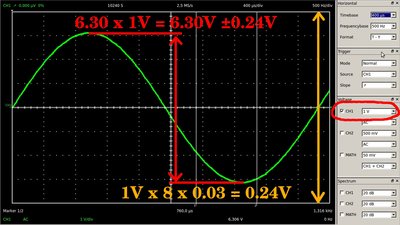
The accuracy of the DSO2090 used in the video is given as 3% from full scale. To get the measurement error, the setting of the axes has to be considered. The maximum reading of the vertical axis is 8 divisions. For an adjustment of 1V per division we get a maximum of 8V, thus the resulting error is 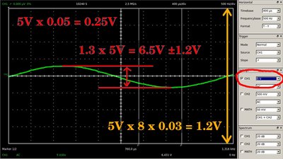
When examining the same input signal at an adjustment of 5V per division, the maximum reading is 40V, thus the resulting error is Trigger
Where should the measurement of a periodically varying signal start? Well, you could start displaying the curve at any point when doing a single measurement, but when repeating the measurement periodically to observe changes in the curve progression, there would be no steady display. 
A logic electrical signal changing status (e. g. 0 to 1) used to initiate a synchronized command to start recording the measurement of an oscilloscope is called trigger. The recording of the curve can be triggered periodically or at certain conditions of the input signal. A periodically triggered recording results in a flipping sine curve (see drawing above), whenever the period of the trigger signal is no integer value of the input signal's period. To get a steady display of the sine wave used here, the measurement has to be started at a certain point of the curve. That could be the point of intersection between the sine curve and the X-axis (=0V) while the voltage is increasing. If that event triggers the recording, we get the red curve. The green curve is displayed, if the recording is triggered at 0V with negative going voltage. The slope switch selects positive-going (red) or negative-going (green) voltage at the selected trigger level. 
At this plot of a square wave signal, the trigger level is set to 1.5V (1V/Div) with negative-going slope. The input signal jumps between 0V and 2V and even small interferences would start the recording while using a 0V trigger level, hence the curve would jump horizontally like the sine wave at the drawing above. With a Digital Storage Oscilloscope (DSO), the plot can also be drawn in reverse direction from the trigger point. At this drawing, the starting point is set to the right of the screen (yellow, vertically pointing arrow) and we can observe the progression of the signal for approximately 1.2 milliseconds (200μs/Div) before the trigger event occurred. 
This plot was recorded with the trigger event set to "single". The oscilloscope starts the recording as soon as the input signal falls below 500mV after rising above that threshold (500mV/Div, negative-going slope) and the recording stops, as soon as the curve reaches the right edge of the screen (after 34ms, 4ms/Div). 40ms of the single event were recorded. You can see the plot of a clap with my hands, recorded with a microphone. To restart the measurement, the oscilloscope must be set to record mode manually. Input resistance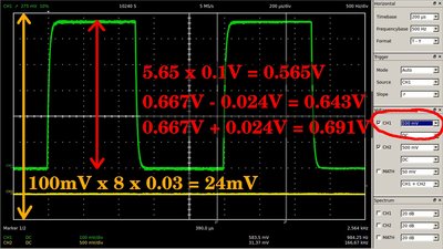
As explained in the chapter about digital multimeters, the input resistance of an oscilloscope has to be considered when recording signals in a high resistive network. The input resistance of the DSO2090 is 1MΩ. The oscilloscope plot shows the signal across resistor number one in a voltage divider composed of three 220kΩ resistors. The chain is connected to a square wave signal with a peak-to-peak voltage of 2V and a frequency of one kilohertz, generated by the oscilloscope. The reading of the peak-to-peak voltage is 5.9 divisions which is 590mV at a vertical adjustment of 100mV/Div. The assumed reading is 
We get a lower reading, because the resistance ratio inside the voltage divider altered. By attaching the probe, an 1MΩ resistor is connected in parallel to the first resistor of the chain. The total resistance of the parallel circuit composed of the oscilloscope and the 220kΩ resistor can be calculated using formula [3.12]: Hence we get a voltage drop at the first resistor of just: Considering the accuracy, the reading should be somewhere between 0.557 and 0.605V which is true for the measured voltage of 0.565V. 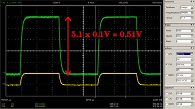
If the second input channel of the oscilloscope is connected in parallel to the first resistor, too, the voltage decreases to just 0.51V. Capacitance
Besides the resistance of the input channel, the capacitance of the cabling and the electric circuits has to be considered when doing measurements with an oscilloscope. The capacitance of the measuring equipment slows down the edge transitions, causing rounded corners at the upper end of the rising edge and the lower end of the falling edge. The coaxial cable of the probe is equivalent to a stretched capacitor and according to the data sheet, the capacitance of the whole unit used in the video is 47 Picofarad. Additionally the capacitance of the electronic circuits of the oscilloscope have to be considered which is listed in the manual of the DSO2090 as 50 picofarad. The animated gif shows the rounded corner at the rising edge of the input signal (green curve). By attaching the second probe to the pin of the test signal (yellow curve), a second capacitor is connected in parallel to the first input channel. As expected, the curve gets rounded even some more. The capacitance of the measurement equipment should be as low as possible. Partial probe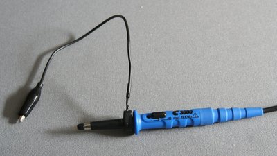
Like any other measuring instrument, oscilloscopes are designed for a certain input range. If the input signal exceeds the maximum input voltage, partial probes can be used to extend the range. A built-in voltage divider forwards just a fixed fraction of the voltage at the tip of the probe to the oscilloscope. The ratio of the probe used in the video is 10:1, hence just one tenth of the voltage at the circuit under test is forwarded to the input channel. The input resistance of the measurement arrangement depends on the resistance of that voltage divider while switched to position "10". The capacitance also changes. The values are listed in the data sheet. The input resistance of this probe is 10MΩ at position "10" and 1MΩ at position "1". The capacitance in position "1" is 47pF and 15.5pF while switched to "10". Maximum resolution
The DSO2090 has an eight bit analog-to-digital converter, hence the analog input voltage can be converted into 256 different digital values. Let's have a look at a linear area of the sine curve generated by an adjustable transformer of a model railway. Instead of a smooth line you can see small steps. At a setting of 5 V/Div, the maximum reading is 35V which is equivalent to 255, the maximum number of the analog-to-digital converter. A single step is equivalent to Sampling rate
Another limitation of an oscilloscope is the number of measurements per second or vice versa, the time needed to capture a single value. At the drawing you can see a square wave signal with a duration of approximately 260ns, recorded with a timebase of 40ns/Div. The signal is displayed with noticeable spikes. That's because the setting of the horizontal axis is at the physical limit of the oscilloscope. The analog-to-digital converter needs 10ns to capture a single value. So there is just one measurement each 10ns, which is equivalent to more than 0.2 divisions at the current setting of the horizontal axis. The software adjustment is clearly below the physical limit of the DSO2090, hence a timebase below 100 nanoseconds is not useful for measurements with that oscilloscope. 10 nanoseconds for a single measurement means that 100 million measurements are done in one second. The sampling rate is 100 megasamples per second (100MS/s). Noise
When examining a DC voltage, a thin horizontal line should appear at the display. At the drawing, the probe is connected to the power pin of an USB port. The DC fraction of the voltage is masked by using the "AC" setting. The vertical adjustment is 10mV/Div. Even if the probe of an oscilloscope is shortened by connecting the ground clamp to the tip of the probe, there is no flat line displayed. One source of error is electromagnetic radiation, which is emitted by nearly all electronic devices. Another source of error is the power supply of the oscilloscope. As demonstrated with the oscilloscope plot, the USB port is no perfect DC power supply. The more the input voltage is smoothened, the better the output signal. The random fluctuation in the displayed input signal is called noise and since that's a characteristic of all electronic circuits including the circuits of the oscilloscope itself it can't be wiped out completely. <<< Current, voltage Rover No.1 >>> News The Project Technology RoboSpatium Contribute Subject index Archives Download Responses Games Links Gadgets Contact Imprint |
|
|