|
|
|
|
News The Project Technology RoboSpatium Contribute Subject index Download Responses Games Gadgets Contact <<< Car design Java-Applet "Tour de Eco" >>> Power balanceThe plots shown below demonstrate the power balances during different driving situations. Considered are the power provided by the automotive engine, the power converted to kinetic and potential energy as well as the power needed to overpower air and rolling resistance. The plots were created using the Java-application "Tour de Eco" at the next page.The test rack consists of a 2km long horizontal section, a 2km long 5% slope, another 2km of horizontal street, a 2km long down grade and finally one more horizontal section of 2km. Once more the values of the project car with combustion engine are used (CW=0,47; A=1,51; CR=0,02; m=765kg=curb weight + half payload; P=17kW). Plotted is the power (y-axis) versus the driven distance (x-axis). The Java-app uses a plotter running permanently from the right to the left and so you can see the driven distance at the end of the x-axis (red circle). Accelerating on a horizontal road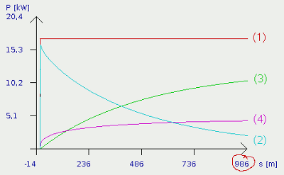
At the starting point, the virtual throttle pedal is kicked down and left at the floor pan for the whole track. Accordingly the red graph (1) bounces up from zero to 17kw. The released engine power doesn't blow out to nowhere but is converted to kinetic and thermal energy. The thermal energy is caused by air and rolling resistance, increasing with car speed. At the beginning, the car is slow whereby just a small amount of power is needed to overpower the resistance. The remaining engine power is transformed into kinetic energy. During the acceleration process at the horizontal street, the sum of kinetic power plus the power needed for air and rolling resistance equals the used engine power. While the speed increases, the power of rolling resistance is growing linear (formula [2.5]) and the power of air resistance is growing cubic (v3, formula [2.16]). Because of the fact that the power is not given versus time but versus distance, the correlations are more complex (which should not confuse us by now). Let's notice that air and rolling resistance grow with higher speeds and so there is fewer engine power left to generate more kinetic energy. As a consequence, the acceleration of our car decreases, but there is always: PMotor (1) = PKin (2) + PAir (3) + PRoll (4) Where is:PAir - power of air resistance, PRoll power of rolling friction, PKin - kinetc power, PMotor - power released by motor 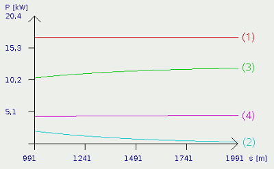
The plots become more and more flattened, the longer the car accelerates and the power used to generate more kinetic energy (2) tends to zero, but will always be different from zero, academically spoken. In practice, the maximum speed of the car will be reached sometime. Using the Java-app, the limit is round about 111km/h. The vehicle registration document lists a maximum speed of 105km/h. Therewith simulation and reality differ just slightly. In practice, the car engine won't release the maximum amount of power at all engine speeds and the engine friction and therewith the power loss, increases with engine speed. This fact is not considered at the simulation. More about the characteristics of an engine will be written at the chapters about electric engines. While speed limit is reached, (PKin=0) there is: PMotor (1) = PAir (3) + PRoll (4) Where is:PAir - power of air resistance, PRoll power of rolling friction, PKin - kinetc power, PMotor - power released by motor Slope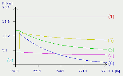
As mentioned above, the car reaches the 5% slope after a distance of 2 kilometers. At the simulation there is a sharp bend in the track and so the power balances alter abrupt. In practice the changeover will always be more smooth, which doesn't influence the balances per se. Who ever has been driving uphill, sitting in a weakly powered car, will have noticed that the maximum speed is clearly lower than on a plane road. The reason for this is the additionally needed power for generating potential energy. At the plot you can see the beginning of the slope clearly. The plot for the power used to overpower air resistance (3) is bent down. Because of the fact that the air resistance is correlated with speed in a cubic way, you can see clearly that the car must be slowing down. Less obvious, but also remarkable is this break at the plot of the power needed to overpower rolling resistance (4). Completely disappeared has the plot of the kinetic power (2), which can be seen at the left, just before the slope was reached. Kinetic energy is generated while the car becomes faster, but the car slows down when reaching the slope. Now we can see the positive effect of kinetic energy: Contrary to the power used to overpower air and rolling resistance, which is lost, the kinetic energy is "buffered". The kinetic energy prevents us from accelerating as well as from slowing down. There is just a small difference - the kinetic power it added to the engine power! Plot (6) was added at the beginning of the slope, showing the inducted kinetic energy. Like shown at formula [2.12], the kinetic energy increases quadratic with car speed hence the support of the engine power by dissipating kinetic energy is smaller, the slower the car becomes. This is the reason why hills can be climbed faster with the right "swing". Also new is the plot for potential power (5). As mentioned, the reason for slowing down lies in generating potential energy, which is also subtracted from the input power (engine power + kinetic power). Potential power is generated whenever a body is lifted towards a restoring force. It should be clear, that a car is lifted while driving uphill. Formula [2.11] shows that the potential energy increases linear with the height. Because of the fact that there is no height difference while driving on a flat road, the power needed to generate potential energy is zero. When reaching the slope, the situation changes abrupt and the according plot bounces up. The gain in potential energy per time interval (=power) is correlated with the car speed. Because of the fact that the car is slowing down, the power used to generate potential power decreases, too. The whole system turns into a stable equilibrium, resulting in a maximum speed for the according slope. With the values given at the simulation, the car is about 82 km/h fast. At a slope, while "slowing down" there is: PAir (3) + PRoll (4) + PPot (5) = PMotor (1) + PKin (6) at equilibrium (PKin=0):PAir (3) + PRoll (4) + PPot (5) = PMotor (1) while accelerating:PAir (3) + PRoll (4) + PPot (5) + PKin (3) = PMotor (1) Where is:PAir - power of air resistance, PRoll power of rolling friction, PPot - potential power, PMotor - motor power At the Plateau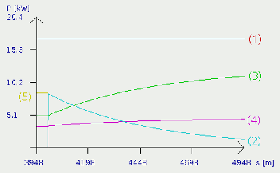
After the 5% slope, a flat section is following. The end of the slope can be seen clearly. Plot number (5) showing the power used to generate potential power disappears (becomes zero), the power of air and rolling resistance start growing and kinetic energy (2) is generated. The relationships mentioned at the beginning of the track can be used to describe the processes. The only difference lies in the fact that the acceleration doesn't start at 0 km/h, but at the final speed of the uphill passage. Decline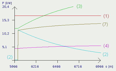
Like the kinetic energy, the potential energy is buffered, too. Power is subtracted from the input power of the system while the car is driving uphill and it is added while the car drives downhill. At the plot you can see clearly that the car starts accelerating again. The plot of the kinetic power (2) bounces up, the power of air and rolling resistance start growing. The reason lies in the appearance of plot number (7), showing the trend of the added potential power. Because of the fact that the car accelerates, it is lowered faster and faster. Therewith the added potential power increases permanently. As you can see, the power to overpower the air resistance (3) becomes higher than the motor power! It "disappears" even at the upper end of the graph. With the simulation data, the maximum speed is about 140km/h! Accelerating at the decline: PAir (3) + PRoll (4) + PKin (2) = PMotor (1) + PPot (7) at equilibrium (PKin=0):PAir (3) + PRoll (4) = PMotor (1) + PPot (7) slowing down:PAir (3) + PRoll (4) = PMotor (1) + PPot (7) + PKin (6) Where is:PAir - power of air resistance, PRoll power of rolling friction, PPot - potential power, PMotor - motor power Another flat section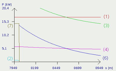
After 8km of the test track passed by, the decline ends and the car is on a horizontal section once again. The plot of the potential power (7) disappears and is not available any longer. According to that, the car is slowing down and kinetic Power is added to the input power. Plot number (6) shows the decreasing kinetic power being applied to the car. Whenever the car is slowing down, the power of air and rolling resistance (3) + (4) are decreasing. The system is running into the equilibrium with the maximum speed of 111km/h. Contrary to the acceleration from 0km/h, the speed is always a little bit higher. Slowing down at the flat section: PAir (3) + PRoll (4) = PMotor (1) + PKin (6) Where is:PAir - power of air resistance, PRoll power of rolling friction, PMotor - motor power Breaking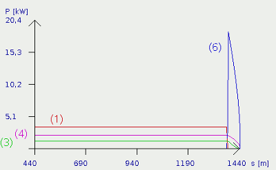
As seen above, kinetic energy may be helpful to climb up hills. The negative aspect of kinetic energy becomes evident while breaking. As well as accelerating, breaking means altering the velocity of a car. Commonly speaking a car accelerates while the absolute value of the velocity is increasing and the car is braking down while the absolute value is decreasing. The point of reference is always the earth's surface. In both cases, work is done and power is needed. Looking at the picture at the left, you can see a breakdown of the car with a speed of round about 15m/s (52km/h) to 0m/s using a constant deceleration. The kinetic power, trying to avoid the slowing down, bounces to ist's highest value at the beginning of the process and decreases faster and faster. The maximum value is even higher than the maximum engine power and this is the reason why our car is slowing down faster than it is accelerating. Like formula [2.12] shows, kinetic energy of the amount ConclusionNow we are able to calculate the amount of energy needed to move a car. Using the benchmarks for the project car has disclosed the weak points. Air and rolling resistance could be optimized to save energy. When dimensioning the batteries, we will see that reducing the mass of the car will be helpful, too.At the next page you will find a "driving simulator", calculating the energy needed to drive a given track. Some remarks on creating your own test tracks for the Java-application: A track consists of up to 100 sections. The sections are numbered () and followed by an equal sign. By the right of the equal sign the length of the section is given. Values from 1 to 10000m are accepted. The length specification is separated from the grade specification by a slash. Values from -20 to 20 are accepted here. Every section has to be terminated by a semicolon (;)! The track is scanned till the first section with the length 0m is reached. A height difference is adjusted by inserting a section with a gradient of +20% or -20% and the according length. Nobody can drive downhill for his whole live... There is no possibility to save the track! Whenever you leave the Java-application, the data is lost. The only way to save the data is to transfer it into a text editor by using " copy & paste". Some examples for tracks: Flat track: (1) = 10000 / 0; Mountain and hill with 15% gradient: (1) = 100 / 0; (2) = 2000 / 15; (3) = 10 / 0; (4) = 2000 / -15; (5) = 100 / 0; (6) = 300 / 15; (7) = 10 / 0; (8) = 300 / -15; (9) = 100 / 0; Mogul slope: (1) = 100 / 0; (2) = 10 / 5; (3) = 10 / 10; (4) = 10 / 15; (5) = 10 / 10; (6) = 10 / 5; (7) = 10 / 0; (8) = 10 / -5; (9) = 10 / -10; (10) = 10 / -15; (11) = 10 / -10; (12) = 10 / -5; (13) = 100 / 0; Play around with the values and try to find out, how much energy is needed to drive a certain distance profile with different speed, different engine power et cetera. The application uses a "electric meter" to display the used energy in kWh. <<< Car design Java-Applet "Tour de Eco" >>> News The Project Technology RoboSpatium Contribute Subject index Archives Download Responses Games Links Gadgets Contact Imprint |
|
|